Chapter 1

Probability begins with a set $\Omega$, called the sample space. Sometimes $\Omega$ is a specified set, but often it does not appear explicitly in computations. The sample space is nevertheless essential in providing a single set where all the events (for example, $\{X\lt 3\}$, $\,\max\{X_t\,|\,t\in[a,b]\}$) are located. Each probabilistic event, such as "the stock price $S_t$ at time $t=3$ is smaller than 100" is a subset of $\Omega$.

It is only natural to require that unions and intersections of events (sets) be allowed, and this gives rise to the need for the events to satisfy some specific properties.

We regularly meet infinite sequences of events, for instance $$ \{X_n\ \le\ 1\}, \quad n=1,2,\dots. $$

What may be observed is that in the definition of $\sigma$-field we only refer to countably infinite unions, and not, for instance, to uncountable unions such as $$ \bigcup_{t\in[0,{1\over2}]}\{X_t\ \le\ 100\}. $$

We will return to the connection between variables (such as $X$) and $(\Omega,{\mathcal F})$ in a little while, after we define the concept of measure. The pair $(\Omega,{\mathcal F})$, where ${\mathcal F}$ is a $\sigma$-field of subsets of $\Omega$, is called a measurable space (a space on which a measure may be defined).

Intervals $(a,b),[a,b),(a,b]$ and $[a,b] $ (with $a\lt b$ ) all have "length" equal to $b-a$; this ordinary length is an example of measure. Let us explain in more detail how the intuitive notion of length is turned into something that agrees with the definition of measure above. First, we define $\Omega=\bf R$ and consider a $\sigma$-field that includes all intervals. The simplest one would be the set of all subsets of $\bf R$. For reasons that go beyond these lecture notes, this is never the $\sigma$-field used. (In short, the set of all subsets of $\bf R$ has too many sets!) A better choice is the " $\sigma$-field generated by the intervals of $\bf R$", the existence of which is justified by the following.

The $\sigma$-field generated by the intervals of $\Reals$ is called the Borel $\sigma$-field over $\Reals$, and is denoted ${\cal B}(\Reals)$. It is indeed strictly smaller than the set of all subsets of $\Reals$, but we will not explain why. There is an infinite number of measures on $(\Reals, {{\cal B}(\Reals)})$, but the most natural measure on $(\Reals, {{\cal B}(\Reals)})$ must be the one we called "length" above: \begin{align}\label{leb} \mu((a,b))\ =\ \mu((a,b])\ =\ \mu([a,b))\ =\ \mu([a,b])\ =\ b-a \end{align} whenever $a\lt b$. This measure is called Lebesgue measure, and will sometimes be denoted $\ell$.

Probability measures are often denoted $\pro$, $\tilde \pro$, $\qpro$, or some similar symbol. The elements of $\Omega$ are often denoted $\omega$.

Random variables

The main reason why random variables are defined the way they will be defined below is that joint distributions are not convenient mathematically when dealing with infinite sets of random variables. If you have one variable, or maybe a small number, then their joint distribution may well be enough, but the joint distribution does not seem to be the right tool to deal with stochastic processes. A better setting has all random variables in the same model represented as mappings from $\Omega$ to $\Reals$.

At this stage there is a similarity between mappings from $\Omega$ to $\Reals$, on the one hand, and the way random numbers are generated in simulation, on the other. In simulation, there are well-known methods for generating random numbers that have a uniform distribution over the interval $(0,1)$. As you have already seen in your previous studies, applications of simulation require many other distributions. For instance, in simulating a continuous-time Markov chain one needs to generate the time the chain spends in the current state, and this time has an exponential distribution.

Most likely you have already learned how to generate a random number having an exponential distribution, if you are given a random number with a ${\bf U}(0,1)$ distribution. If a variable $U$ has a ${\bf U}(0,1)$ distribution, then $Y_1=-\log U$ has an ${\bf Exp}(1)$ distribution; $Y_1$ is a function of $U$, that we could write $Y_1=g(U)$. Here is another example. Define $Y_2=\sqrt U$. Then $Y_2$ has a ${\bf Beta}(2,1)$ distribution. The two variables $(Y_1,Y_2)$ have a joint distribution that can be calculated. Nothing prevents us from defining any number of variables $Y_1,Y_2,Y_3,\dots$ as functions of the same variable $U$. This can be done in simulation, but in the the mathematical theory of probability this is fundamental, as we now show.

In all applications of stochastic processes, there is a set $\Omega$ and any variable $X$ is a mapping (= function) from $\Omega$ to the set of real numbers: $$ X:\,\Omega\ \to\ \Reals. $$ To emphasize the parallel with simulation, imagine that $\Omega=(0,1)$ and that the function is $$ X(\omega)\ =\ -\log\, \omega, \quad \omega \in(0,1). $$ A moment's reflection makes one realize that this is not enough to have randomness, since there is yet no probability distribution anywhere. The parallel with simulation makes it clear that $X$ will have a probability distribution if there is a probability distribution ("measure") for the $\omega$'s (which replace $U$ here). The vocabulary and notation here is as follows: "let $\Omega$ be a set, ${\mathcal F}$ be a $\sigma$-field of subsets of $\Omega$, and $\pro$ be a probability measure over $(\Omega,{\mathcal F})$". Suppose $X$ associates a real number to each $\omega\in\Omega$; then the probability measure on $\Omega$ gives the real numbers $X(\omega)$ a probability distribution. In other words, the "state of the world" $\omega$ is chosen randomly according to the probability measure $\pro$, and thus $X(\omega)$ is also random. The situation may be summarized as follows: $$ \{\text{prob. measure over }\Omega \}\ \to\ \{\text{mapping $X$}\} \ \to\ \{\text{distr. of } X\text{ over }\Reals\}. $$ This is not so difficult to understand. What may be less obvious is that in actual modelling, when we use one or more stochastic processes, we always assume the above setup but we rarely specify $\Omega$ or $\pro$. The pair $(\Omega,\pro)$ is absolutely essential, but once we know the structure of the system and its properties we do not always need to specify all its parts.

In order to illustrate what is happening, we will assume that $\Omega=(0,1)$ and that $\pro$ is the uniform probability measure (= Lebesgue measure) over $\Omega$. Any random variable $X$ is a mapping from $\Omega$ to $\Reals$, and the distribution of $X$ is found from $$ \pro(X\in B)\ \mathop{=}^{\text{def}}\ \pro\{\omega\,\left|\,X(\omega)\in B\}\right.,\quad B\ \text{a subset of }\Reals. $$ This is just the same as in the simulation example: if it is known that $U\sim U(0,1)$ and we then define $Y=-\log U$, we find, for example, $$ \pro(Y\gt1)\ =\ \pro(Y\in (1,\infty))\ =\ \pro(\log U\lt-1)\ =\ \pro(U\lt e^{-1})\ =\ e^{-1}. $$ In order to find the distribution of $Y$ we need to "go back" from the set where $Y$ takes its values, namely $\Reals$, to the set where $U$ takes its values, namely $(0,1)$. The distribution of $U$ is transformed by the mapping $Y$, and the result is the distribution of $Y$.

In probability and statistics, $\pro$ "lives" on the set of subsets of $\Omega$, and the distribution of $X$ "lives" on the set of subsets of $\Reals$, and the latter is found from the former by going back from $\Reals$ to $\Omega$: \begin{align*} \Omega\quad &\mathop{\longrightarrow}^{X}\quad \Reals\\ \pro\quad &\mathop{\longrightarrow}^{X}\quad F_X(\cdot). \end{align*} In order for $F_X(x)$ to be well defined, the event (= subset of $\Omega$) $$ \{\omega\in\Omega\,|\, X(\omega)\le x\} $$ must be "legitimate", in the sense that it is an element of ${\mathcal F}$. This leads to the requirement: \begin{align}\label{rv} \text{for all }\ x\in\Reals,\quad \{\omega\in\Omega\,|\, X(\omega)\le x\}\in{\mathcal F}. \end{align} This can be taken as the definition of a random variable, but mathematicians more often use a condition that is worded differently but is equivalent.

This condition includes \eqref{rv}, since $$ \{\omega\in\Omega\,\left|\, X(\omega)\le x\}\right.\ =\ \{\omega\in\Omega\,\left|\, X(\omega)\right.\in(-\infty, x]\}, $$ and $(-\infty,x]$ is an element of the Borel $\sigma$-field ${\cal B}(\Reals)$. It can be shown that \eqref{rv} and \eqref{rv1} are the same.

However, the terminology is again a little strange, since the definition of random variable does not involve randomness at all! A mapping $X$ is a random variable if it has the right property regarding the sets $\{\omega\in\Omega\,\left|\, X(\omega)\in B\}\right.$, $B\in{\cal B}(\Reals)$.

More on terminology: a random variable is the same as a measurable mapping, or measurable function. In the next subsection we talk of measurable functions in order to include integration with respect to measures, not just probabilities.

$\sigma$-field generated by a random variable

If $X$ is a random variable, the smallest $\sigma$-field that contains all the events $\{\{X\le x\},\,x\in\Reals\}$ is called the $\sigma$-field generated by $X$, and is denoted $\sigma(X)$.

Integration

Why talk of integration? You already know about \begin{align}\label{int} \int_a^b f(x)\,dx \end{align} for a large class of functions $f(\cdot)$, so what else could be needed? In the end, the new definition of integral we give below will not change the values of the expectations we will compute, but:

A probability measure is often denoted $\pro$ or $\qpro$, and the integral of a measurable function (= random variable) $X$ is written $\int X\,d\pro$, and so on, but the definition of the integral is the same as for integration with respect to a measure.

It can be shown that every non-negative measurable function $f(\cdot)$ is the limit of a non-decreasing sequence of step functions $\{f_n,n\ge1\}$. This is obvious when $\Omega$ is the interval $[a,b]$ and $f$ is continuous; but the fact is also true for $f$ that is just measurable, even though measurable functions can have discontinuities, even an infinite number of them! The integral of $f$ is then the limit of the integrals of the step functions.

In symbols, a step function $g$ is written as $$ g(x)\ =\ \sum_{j=1}^{K}\alpha_j{\bf1}_{A_j}(x), $$ where $A_j\cap A_k=\emptyset$ for $j\ne k$ and $\displaystyle \bigcup_{j=1}^{K}A_j=\Omega$ (the sets $\{A_1,\dots,A_{K}\}$ form a partition of $\Omega$), and $\{\alpha_j\}$ are constants. The integral of $g$ with respect to a measure (or probability measure) $\mu$ on $(\Omega, {\mathcal F})$ is defined as:

For arbitrary functions $f$ the integral $\int f\,d\mu$, if it exists, is defined by taking limits of integrals of step functions $g_n$ that converge to $f$ as $n$ tends to $\infty$ (we omit the details). Below we will mention one case where the integral does not exist.

A couple of comments. First, the integral of $f$ may be $+\infty$. Second, the integral of $f$ over a subset $A$ of $\Omega$ is defined as the integral of $f$ times the indicator function of $A$: $$ \int_Af\,d\mu\ \mathop{=}^{\text{def}}\ \int f{\bf1}_A\,d\mu\ =\ \int f(\omega){\bf1}_A(\omega)\,d\mu(\omega). $$ Third, what about the good old Riemann integral $$ \int_a^b f(x)\,dx $$ that you learned about in previous courses? The theory of Lebesgue integration that was very briefly outlined above is not absolutely identical with Riemann integration over $\Reals$, but in computing integrals numerically you may never notice the difference. The Riemann integral of $f$ over the interval $[a,b]$, if it exists, is the same as the integral of the function $f{\bf1}_{[a,b]}$ with respect to Lebesgue measure. The latter is the measure that assigns length to intervals, as we noted already. If we want to differentiate Riemann and Lebesgue then it is customary to use a symbol, for instance $\ell$, to denote Lebesgue measure, and write $$ \text{Riemann:}\quad \int_a^b f(x)\,dx,\quad \text{Lebesgue:}\quad \int_{[a,b]} f(x)\,d\ell(x). $$ We will not need to do this in this book. When we write $\displaystyle \int_a^b f(x)\,dx$ we mean the Lebesgue integral, which, in calculations, will end up being the same as the Riemann integral, or "area under the curve".

N.B. So when would the two be different? There are cases where a Riemann integral over a finite interval may fail to exist, while the Lebesgue will exist, here is an example. Suppose $f(x)$ equals 1 if $x$ is rational, and $0$ otherwise; the Riemann integral of this function over some finite interval does not exist, since the "upper sums" and "lower sums" do not have the same limits; however, the Lebesgue integral of that function does exist, and equals 0, because the set of rational numbers is countable. This type of situation does not arise explicitly in this book.

Expectation of a random variable

The expectation of a random variable can now be defined in terms of the probability measure $\pro$ over $(\Omega,{\mathcal F})$ (the distribution of $X$ over $\Reals$ is not needed here): recalling that a random variable is simply a measurable mapping over $(\Omega,{\mathcal F})$, one defines

Here is a simple example, to fix ideas. Suppose $\Omega=(0,1)$, ${\mathcal F}$ is the Borel $\sigma$-field over (0,1) (again this is the $\sigma$-field generated by the intervals included in (0,1)), the probability $\pro$ is the uniform probability over (0,1), that is the probability that assigns $$ \pro((a,b))\ =\ b-a,\quad 0\lt a\lt b\lt 1. $$ (This is Lebesgue measure restricted to the interval (0,1).) Then $$ \esp X\ =\ \int X\,d\pro\ =\ \int_0^1 X(\omega)\,d\omega. $$ For instance, if $X(\omega)=-\log\omega$, then this is $$ -\int_0^1\log \omega\,d\omega\ =\ -\Big[\omega\log\omega-\omega\Big]_{\omega=0}^{\omega=1}\ =\ 1. $$ (Note we caclulated this just as though it was a Riemann integral.) In this case $ |X(\omega)|=X(\omega)$, so this also checks that $\int |X|\,d\pro\lt \infty$.

The distribution of $X$ is found as follows. The possible values of $X$ are between zero and infinity, so let $x\in(0,\infty)$:

You will recall that in other courses the expectation of $X$ was was (most likely) defined as $$ \int_0^\infty xe^{-x}\,dx\ =\ 1. $$ It is reassuring to find the same answer, but is this always going to be the case? There now appear to be two different ways of computing expectations! For continuous random variables $X$, the two contenders are: $$ \text{old formula:}\quad \int_{-\infty}^\infty xf_X(x)\,dx,\q\dots\q \text{new formula:}\int X\,d\pro. $$ Which is the "true" expectation? What connects the dots?

What makes the two integrals equal is that the density of $X$ can be obtained from $\pro$: $$ F_X(x)\ =\ \pro\{\omega\,|\,X(\omega)\le x\},\q\q f_X(x)\ =\ {d\over dx}F_X(x). $$ The two integrals are the same because one can be obtained from the other by a change of variable, as explained in the following theorem.

The law of the unconscious statistican

Theorem 2. Suppose $X$ is a random variable on the probability space $(\Omega,{\mathcal F},\pro)$ that has a finite expectation $$ \esp X\ =\ \int X\,d\pro. $$ Then this expectation is the same as the "distributional" expectation of $X$ calculated with respect to the distribution of $X$ over $\Reals$, in particular, if $\esp X$ exists, then, for a continuous random variable $X$, $$ \esp X\ =\ \int_{-\infty}^\infty xf_X(x)\,dx, $$ and for a discrete random variable $X$, $$ \esp X\ =\ \sum_{\textit{possible values}\ x_k}x_k\pro(X=x_k). $$

We will not prove this theorem, but here is the justification in the example above. Take the new definition of the expectation

Theorem 2 above says that this change of variable works every time. There often is a real advantage in not working with the distribution of $X$, for instance in cases where that distribution is unknown (or is of no importance!). Another very significant advantage is having no restriction of the number of variables involved in an expectation. For instance, if $\{W_t,t\ge0\}$ is a Brownian motion, then $$ \esp \max_{0\le t\le 1}W_t $$ involves an infinite number of variables.

Lebesgue integrals have the following two fundamental properties, that are among the most useful theorems of probability theory: the Dominated Convergence Theorem, and the Fubini Theorem.

Integrable functions (mappings, variables)

Some mappings are integrable, others are not. For instance, the mapping $-\log \omega$ we saw above is integrable with respect to the Lebesgure measure, denoted "$\ell$", on $\Omega=(0,1)$; the same mapping may or may not be integrable with respect to other measures defined on the same space $(\Omega,\calf)$, one needs to check every case individually.

If $a>1$, then $$ \int Y\,d\pro\ =\ \int_0^1 \omega^{-{1\over a}}\,d\omega\ =\ {a\over a-1}. $$ The reader will check that for $0\lt a\le1$ the result is $\infty$. In those cases the mapping $Y$ is not integrable; since $Y$ is a random variable, this is the same as saying that the variable $Y$ is not integrable. We say that the expectation of $Y$ is infinite. We will do the same each time a variable $X$, which takes non-negative values, is such that $\esp X=\infty$. Observe that any random variable $Y$ has absolute value $X=|Y|\ge0$; hence, for any variable $Y$ there are only two possibilities, either $\esp |Y|\lt \infty$, or $\esp |Y|=\infty$. Of course "$\infty$" is not a number, so in the second case the expectation of $|Y|$ "does not exist". When dealing with non-negative variables it is probably easier to stick to using the words "integrable" (expectation of $|Y|$ is finite) or "not integrable" (expectation of $|Y|$ is infinite), rather than saying that the expectation of $|Y|$ "exists" or "does not exist".

Example.. The Cauchy distribution has probability density function $$ f(x)\ =\ {1\over \pi}{1\over 1+x^2},\quad x\in\Reals. $$ In order to talk of the expectation of this variable, we first need to check that $$ \int_{-\infty}^\infty |x|f(x)\,dx\ \lt\ \infty. $$ Split the integral into two in the obvious way (from minus infinity to 0, and from 0 to plus infinity). The two integrals have the same value (why?). We see that \begin{align} {x \over1+x^2}\ \approx\ {1\over x} \end{align} for large $x$, and we know that $$ \int_1^\infty {dx\over x}\ =\ \infty. $$ The area under $\displaystyle {1\over x}$ is infinite; that curve is very close to $\displaystyle {x\over 1+x^2}$ for large $x$, which leads us to suspect that the area under the second curve might also be infinite. In this case we actually can integrate the function exactly over $(0,\infty)$: \begin{align} \int_0^\infty {x \over1+x^2}\ ={1\over2}\log (1+x^2){\Big|}_{x=0}^{x=\infty}\ =\ \infty. \end{align} Hence, any variable $X$ with a Cauchy distribution is not integrable. In this case we cannot write "$\esp X=\infty$", because, by a simple change of variable, $$ \int^0_{-\infty} xf(x)\,dx\ = \ -\int_0^{\infty} xf(x)\,dx\ =\ -\infty, $$ and thus $$ \int_\Reals xf(x)\,dx\ =\ \int_0^\infty+\int_0^{\infty} \ =\ "\infty-\infty". $$ The last expression is undefined in mathematics. When this happens we say that the expectation of the variable is undefined.

In conclusion, there are three possibilities: an expectation is finite, infinite ($+\infty$ or $-\infty$), or undefined.

Integrating over sets of measure (or probability) zero

A few words on these expressions. Sets of zero measure, or zero probability, are present everywhere in the theory and application of stochastic processes, which is why the "a.e", "w.p.1" and "a.s." need to be added to many identities between random variables, such as "$X=Y$ a.s.". For instance, the Lebesgue measure of a single point is zero. One way to see this is as follows. To begin with, the set $\{b\}$ is in ${\mathcal B}(\Reals)$, since both $(a,b]$ and $[b,c)$ are ${\mathcal B}(\Reals)$ and $$ (a,b]\ =\ \cap(a,b)\cup \{b\} $$ (assuming $a\lt b$). Then, if $\ell$ stands for Lebesgue measure, recalling its defining property \eqref{leb}, $$\eqalign{ b-a\ &=\ \ell((a,b])\ =\ \ell((a,b)\cup\{b\})\cr &=\ \ell((a,b))+\ell(\{b\})\cr &=\ b-a+\ell(\{b\}), } $$ which implies $\ell(\{b\})=0$. Hence, if $A\subset \Reals$ is a finite or countable set $\{b_1,b_2,\dots\}$ then it is in ${\mathcal B}(\Reals)$ and, from the definition of measure, $$ \ell(A)\ =\ \sum_k\ell(\{b_k)\}\ =\ 0. $$ The consequence is that the integral with respect to Lebesgue measure of any function over a countable set is zero: $$ \int_{\{b_1,b_2,\dots\}} f(x)\,dx\ =\ 0 $$ Another consequence is that changing the values of a function at a finite or countable number of points does not change the value of its integral with respect to Lebesgue measure. For instance, if \begin{align*} \phi(x)\ =\ {e^{-{x^2\over2}}\over\sqrt{2\pi}},\quad\quad g(x)\ =\ \begin{cases} \phi(x),&x\notin \Integers\\[2pt] \phi(x)+10^{10^{10}},& x\in\Integers\end{cases} \end{align*} then $$ g(x)-\phi(x)\ =\ 10^{10^{10}}{\bf1}_\Integers(x) $$ and thus $$ \int_{-\infty}^\infty g(x)\,dx\ =\ \int_{-\infty}^\infty\phi(x)\,dx+\int_{-\infty}^\infty (g(x)-\phi(x))\,dx\ =\ 1+ \int_\Integers 10^{10^{10}}\,dx\ =\ 1. $$ The same happens for all measures or probability measures that have a density, for instance $$ \pro((a,b))\ =\ \int_{(a,b)\cap \Reals_+}e^{-x}\,dx. $$ In all such cases the integral over a countable set is zero: $$ \int_{\{b_1,b_2,\dots\}} f(\omega)\,d\pro(\omega)\ =\ 0. $$ Of course the situation is different for probability measures that have a "discrete" part, for instance the probability measure $$ \qpro(\{k\})\ =\ {6\over \pi^2}{1\over k^2},\quad k\ =\ 1,2,\dots, $$ has all its mass on the countable set $\Naturals$; here the probability of a finite or countable set is positive if the set contains at least one positive integer. The notation needs getting used to: integrating with respect to a discrete measure really means performing a sum; for example, the mapping $X(k)=k$ has infinite expectation, under the measure $\qpro$: $$ \esp X\ =\ \int X\,d\qpro\ =\ \sum_{k=1}^\infty k\qpro(\{k\})\ =\ \infty. $$

Dominated Convergence Theorem

The first of the two fundamental theorems we will use in this book (and that are regularly used financial mathematics) is the Dominated Convergence Theorem, which give a simple condition that guarantees that "the limit of the integrals equals the integral of the limit". The need for such a result is illustrated in the following example.

Example Suppose the functions $\{f_n(x),\,n=1,2,\dots\}$ are defined as $$ f_n(x)\ =\ n(1-nx){\bf1}_{(0,{1\over n})}(x), \quad f(x)\ =\ 0. $$ The graphs are triangles that get taller when $n $ increases, while the base gets narrower. The area under the curve is $1\over2$ for all $n$, but because the indicator function ${\bf1}_{(0,{1\over n})}(\cdot)$ shrinks to nothing as $n$ tends to infinity, we see that $$ \lim_{n\to\infty}\int_\Reals f_n(x)\,dx \ =\ {1\over2};\q \int_\Reals \lim_{n\to\infty}f_n(x)\,dx \ =\ \int_\Reals 0\,dx \ =\ 0. $$

The Dominated Convergence Theorem below refers to "almost sure" convergence of a sequence of random variables, and as pointed out above in the case of integrals this is convergence that happens "everywhere with the possible exception of a set of probability zero".

Theorem 4 (Dominated Convergence Theorem, or Dominated Convergence Theorem). Suppose $\{X_n,n\ge1\}$ are random variables defined on a probability space $(\Omega,{\mathcal F},\pro)$, that converge almost surely to a random variable $X$; this means that there is a set $A\in {\mathcal F}$ with $\pro(A)=1$ such that $$ \lim_{n\to\infty}X_n(\omega)\ =\ X(\omega), \quad \omega\in A. $$ If there exists another random variable $Y\ge0$ that is integrable with respect to $\pro$, i.e. $$ \esp Y \lt \infty, $$ and such that $$ |X_n(\omega)|\ \le\ Y(\omega),\quad \omega\in A, $$ then (a) each $X_n$ is integrable with respect to $\pro$, and (b) $$ \lim_{n\to\infty}\esp X_n\ =\ \esp X. $$

Note that a Dominated Convergence Theorem is part of the Dominated Convergence Theorem, which says that if $Y$ is integrable and $|X(\omega)|\le Y(\omega)$ a.s., then $X$ is also integrable.

Example. A classic application of the Dominated Convergence Theorem is the following. Suppose $\{Z_n,\,n\ge1\},\,Z$ are random variables, and consider the characteristic functions $$ \psi_n(p)\ =\ \esp e^{ipZ_n},\quad \psi(p)\ =\ \esp e^{ipZ}. $$ Here $i$ is the imaginary unit ($i^2=-1$) and $p\in\Reals$. The characteristic function always exists, because $$ |e^{iy}|\ =\ |\cos y+i\sin y|\ =\ \sqrt{\cos^2y+\sin^2y}\ =\ 1 $$ if $y\in\Reals$. Characteristic functions are essential in the study of probability distributions; they are more useful than moment generating functions because the latter do not always exist. The Dominated Convergence Theorem yields an important property of characteristic functions, namely that if $Z_n$ converges to $Z$ almost surely, then $\psi_n(p)$ converges to $\psi(p)$ for all $p\in\Reals$. The detailed reasoning is as follows: by assumption there is a set $A$ with $\pro(A)=1$ such that if $\omega\in A$ then $$ \lim_{n\to\infty}Z_n(\omega) \ =\ Z(\omega). $$ Therefore $$ \lim_{n\to\infty}e^{ipZ_n(\omega)} \ =\ e^{ipZ(\omega)} $$ for each $\omega\in A$, meaning that the variables $X_n=e^{ipZ_n}$ converge almost surely to $X=e^{ipY}$, and, moreover, $|X_n(\omega)|\le Y(\omega)=1$. The variable $Y$ is integrable. Finally, the Dominated Convergence Theorem may be applied, and \[\lim_{n\to\infty}\esp X_n\ =\ \lim_{n\to\infty}\psi_n(p)\ =\ \esp X=\psi(p).\]

Fubini's Theorem

Theorem 5 (Fubini's Theorem). Suppose two measure spaces $(\Omega_j,{\mathcal F}_j,\mu_j)$, $j=1,2$.

(a) If $f(x,y)\ge0$ for all $(x,y)$, then \begin{align}\label{fub} \int_{\Omega_1}\left[\int_{\Omega_2}f(x,y)\,d\mu_2(y)\right]d\mu_1(x)\ =\ \int_{\Omega_2}\left[\int_{\Omega_1}f(x,y)\,d\mu_1(x)\right]d\mu_2(y). \end{align} This is true whether the double integrals are finite or infinite.

(b) Another sufficient condition for \eqref{fub} to hold is \[\displaystyle \int_{\Omega_1}\left[\int_{\Omega_2}|f(x,y)|\,d\mu_2(y)\right]d\mu_1(y) \lt\infty. \] In this case it is not required that $f(x,y)\ge0$ for all $(x,y)$, and the double integrals in \eqref{fub} are necessarily finite.

Examples. 1. A result that is used very often in applications is: "if $X$ is non-negative then $$ \esp X\ =\ \int_0^\infty \pro(X>x)\,dx. $$ The proof is based on Fubini's Theorem. First, write $$ X\ =\ \int_0^X\,dx\ =\ \int_0^\infty {\bf1}_{\{X>x\}}\,dx. $$ Next, $$ \esp X\ =\ \esp \int_0^\infty {\bf1}_{\{X>x\}}\,dx\ =\ \int_\Omega \left[ \int_{\Reals_+} {\bf1}_{\{X(\omega)>x\}}\,dx \right]d\pro(\omega). $$ Here $X$ is a random variable on the probability space $(\Omega,{\mathcal F},\pro)$, and the other measure space is $(\Reals_+,{\mathcal B}(\Reals_+),\ell)$, where $\ell$ is Lebesgue measure on $\Reals_+$. The function of two variables being integrated is $$ f(\omega,x)\ =\ {\bf1}_{\{X(\omega)>x\}}. $$ The first part of Fubini's Theorem says that the order of integration may be reversed, since $f(\omega,x)\ge0$. Therefore, $$ \esp X\ =\ \int_{\Reals_+}\left[ \int_\Omega {\bf1}_{\{X(\omega)>x\}}d\pro(\omega) \right] \,dx \ =\ \int_{\Reals_+} \esp {\bf1}_{\{X>x\}}dx\ =\ \int_{\Reals_+} \pro(X>x)dx. $$ Note that this is true for any type of distribution, discrete, continuous, mixed or singular.

2. A situation encountered several times in this book (and also in financial mathematics more generally) concerns the expectation of the integral of a stochastic process, specifically suppose we know $\esp X_s$ for each $s$, and we wish to $$ \text{find}\ \ \esp I\ \ \text{if}\ \ I\ =\ \int_0^t X_s\,ds. $$ The question is: is it always true that \begin{align}\label{I} \esp I\ =\ \int_0^t \esp X_s\,ds? \end{align} The answer is "no", but Fubini's Theorem gives two sufficient conditions for this to be the case. The expectation of $I$ can be written $$ \esp I\ =\ \int_\Omega \left[ \int_{[0,t]} X_s(\omega)\,ds \right]d\pro(\omega). $$ There are two measure spaces, $(\Omega,{\mathcal F}, \pro)$ and $([0,t], {\mathcal B}([0,t]),\ell)$, where $\ell$ is Lebesgue measure restricted to $[0,t]$. The first part of Fubini's Theorem says that if $X_s(\omega)\ge0$ for all $\omega\in\Omega$ and $s\in[0,t]$, then $$ \int_\Omega \left[ \int_{[0,t]} X_s(\omega)\,ds \right]d\pro(\omega)\ =\ \int_{[0,t]} \left[\int_\Omega X_s(\omega)d\pro(\omega) \right]ds\ =\ \int_{[0,t]} \esp X_s\,ds $$ and \eqref{I} holds.

Remark. There is more to Fubini's Theorem. Theorem 5 only refers to iterated integrals, that is to double integrals that are calculated one variable at a time. For instance, the way the iterated integral $$ \int_{\Omega_2}\left[\int_{\Omega_1}f(x,y)\,d\mu_1(x)\right]d\mu_2(y) $$ is written means that one would first calculate the inner integral $$ \int_{\Omega_1}f(x,y)\,d\mu_1(x) $$ for each $y$, and then integrate the resulting function of $y$, say $$ g(y)\ =\int_{\Omega_1}f(x,y)\,d\mu_1(x) $$ with respect to $\mu_2(y)$, in effect calculating $$ \int_{\Omega_2}g(y)\,d\mu_2(y). $$ Theorem 5 gives conditions under which one can start integrating with respect ot $x$ or $y$ without altering the result of the iterated integration. The full version of Fubini's theorem also refers to the double integral as seen as a single integral with respect to the product measure $\mu_1\times \mu_2$, calculated over the product space $\Omega_1\times\Omega_2$. We omit the details.

Types of probability distributions

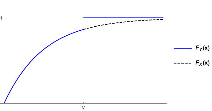
There are probability distributions that are not continuous nor discrete. Here is an example.

Example. In some statistical experiment, it is only possible to measure $X$ exactly up to a value $M$; when $X>M$ then the value $M$ is recorded. Hence, what is observed is not $X$ but \begin{align} Y\ =\ \begin{cases}X&\text{if } X \lt M\\[3pt] M&\text{if } X\ge M. \end{cases} \end{align} (This is called censoring in statistics.) Suppose $X\sim{\bf Exp}(1)$ and that $M$ is a positive constant. What is the probability distribution of $Y$? We find \begin{align} F_Y(x)\ =\ \pro(Y\le x)\ =\ \begin{cases}\pro(X\le x)\ =\ 1-e^{-x}&\text{if }x\lt M\\[3pt] 1&\text{if }x\ge M. \end{cases} \end{align} A graph of the distribution functions $F_X(\cdot)$ and $F_Y(\cdot)$ is provided. The variable $Y$ does not have a continuous distribution , since $\pro(Y=M)=e^{-x}>0$. It does not have a discrete distribution either, because there is no finite or countable set $V$ such that $\pro(Y\in V)=1$.

The variable $Y$ has a distribution of the mixed type. A variable $Z$ with a mixed distribution has a finite or countable set $V$ such that $\pro(Z\in V)\in(0,1)$, and there is at least one interval $(a,b)$ where $$ {d\over dx}\pro(Z\le x)\ >\ 0. $$

Simulation

A common technique for simulating random numbers is the inverse transform method. For a specific distribution function $F(\cdot)$, one generates random numbers $U_1, U_2,\dots$, with a ${\bf U}(0,1)$ distribution, and then applies a function, say $g(\cdot)$ to $U_k$ that is such that $g(U_k)$ has the specified distribution. There is a theorem that says that for any distribution function $F(\cdot)$ there is a $g(\cdot)$ such that $X=g(U)$ which has that distribution function, given $U\sim\,{\bf U}(0,1)$. We look at particular cases of this theorem in the exercises.